Visualizing dead-end roads in cities.
Have you ever been stuck in traffic, wondering why seemingly everyone is going where you’re going?
Often, the problem isn’t just the sheer number of cars. It’s suburban and urban layout design.
Years ago, I stumbled upon a study examining the ratio of dead-end roads to total road network length and how directly it correlates with traffic congestion:
traffic_congestion = dead_end_roads / total_roads
When neighborhoods rely heavily on culs-de-sac and branching dead-ends,
traffic cannot diffuse naturally through parallel streets.
Instead, every vehicle is funneled onto a handful of high-capacity through-ways:
                     ▲
         ──────┐     ║     ╔══════╗
               │     ║     ║      ║
          ┌────┴─────╣     ║      ║
          │          ║     ║      ║
     ─────┘          ╠═══╦═╝      ║
        ──┬───┐      ║   │        ╚═══╗   ┌─────
          │   │      ║   │            ║   │
          │   └──────╣   │   ────┐    ║   │
          │          ║           │    ║   │
          │          ║           └────╬───┘
          │          ║                ║
                     ╠════════════════╣
──────┬─────┐        ║                │
      └─────┴────────╣                │
                     ║                │
                     ║
                     ▼
-- dead-end
== through-way
▼ External boundary connection
Conversely, grid-like or highly interconnected networks distribute vehicles across multiple redundant paths, dampening overall congestion:
                   ▲
   ╔═══════╗       ║       ╔════╗
   ║       ║       ║       ║    ║
   ║    ╔══╩═══════╣       ║    ║
   ║    ║          ║       ║    ║
   ╚════╣          ╠══╗════╝    ║
    ┌───╬════╗     ║  ║         ╚═══╗   ┌─────
────┘   ║    ║     ║  ╚════════╗    ║   │
        ║    ╚═════╣           ║    ║   │
        ║          ║           ║    ║   │
        ║          ║           ╚════╬───┘
        ║          ║                ║
        ║          ╠════════════════╝
        ╚════╗     ║
  ───────────╩═════╣
                   ║
                   ║
                   ▼
-- dead-end
== through-way
▼ External boundary connection
The original study analyzed abstract cities I had never visited. I wanted to see how these dynamics played out in the towns and cities I actually drive through!
Designing the Algorithm
To map these bottlenecks, I needed an algorithm capable of taking any geographical boundary, pulling its street network, and identifying every road segment that functions as a dead-end.
I broke the problem down into three primary stages:
1. Data Collection & Caching
Using OpenStreetMap via the Overpass API, I queried road network data for selected regions and cached the raw spatial data locally as graph nodes (intersections/bends) and edges (road segments).
(Later in the project, I switched to downloading raw .obf files for entire OSM regions—a massive efficiency boost over API requests.)
2. Topological Simplification
Raw GIS data contains nodes for every subtle curve in a road. For graph analysis, mid-block geometry is noise. I collapsed linear chains of nodes into single edges, keeping only actual junctions and terminal points:
       ▲
    ─┴─╣
       ╠═╦═╗
       ║ │ ║
    ─┬─╣  ─╬─
       ╠═══║
   ┌┬──╣   │
  ─┴┘  ▼
-- dead-end
== through-way
▼ External boundary connection
3. Identifying Graph Bridges
Translating urban geography into graph theory simplifies the core logic:
A dead-end road network is bounded by a “bridge” in graph theory.
A bridge is an edge whose removal splits a connected graph into separate components. Any road segment downstream of a bridge leads exclusively to dead-ends.
                     ▲
         ──────┐     ║     ╔══════╗
               │     ║     ║      ║
          ┌────┴───X─╣     ║      ║
          │          ║     ║      ║
     ─────┘          ╠═══╦═╝      ║
        ──┬───┐      ║   │        ╚═══╗   ┌─────
          │   │      ║   │            ║   │
          │   └──────╣   │   ────┐    ║   │
          │          ║           │    ║   │
          │          ║           └────╬───┘
          │          ║                ║
                     ╠════════════════╣
──────┬─────┐        ║                │
      └─────┴────────╣                │
                     ║                │
                     ║
                     ▼
-- dead-end
== through-way
▼ External boundary connection
X A bridge
Handling External Boundary Connections
Without accounting for roads that exit the bounding box, major arterial highways passing through the region would be falsely flagged as bridges.
To fix this, the algorithm attaches every perimeter-crossing exit node to a virtual “World” node:
                     ═ ═ ═ ═ ═ ═ ═ ═ ═ ═ ═ ═ ═ ═ ═ ═
         ──────┐     ║     ╔══════╗                ║
               │     ║     ║      ║
          ┌────┴─────╣     ║      ║                ║
          │          ║     ║      ║
     ─────┘          ╠═══╦═╝      ║                ║
        ──┬───┐      ║   │        ╚═══╗   ┌─────
          │   │      ║   │            ║   │        ║
          │   └──────╣   │   ────┐    ║   │       ┌──────┐
          │          ║           │    ║   │       │World │
          │          ║           └────╬───┘       └──────┘
          │          ║                ║            ║
                     ╠════════════════╣
──────┬─────┐        ║                │            ║
      └─────┴────────╣                │
                     ║                │            ║
                     ║
                     ═ ═ ═ ═ ═ ═ ═ ═ ═ ═ ═ ═ ═ ═ ═ ╝
-- dead-end
== through-way
= = = Virtual edge joining boundary exits to the World node
Because external exits loop through the World node, arterial routes maintain alternative connectivity paths, ensuring only true dead-end pockets are flagged.
From Ruby Prototype to Rust Engine
My initial prototype was written in Ruby. While easy to draft, it was computationally heavy and memory-bound. It handled tiny sub-neighborhoods (~25 sq km) reasonably well, but attempting to process an entire city resulted in minutes of processing before eventually running out of memory.
Recently, I revisited the project and ported the graph engine to Rust (with assistance from LLM code generation for the graph traversal boilerplate). The performance leap was dramatic: execution times dropped from minutes to milliseconds, allowing seamless parsing of full metropolitan transit networks, and the ability to process whole countries in under a minute!
Findings & Map Visualizations
Comparing street networks across different regions highlights how urban planning paradigms directly dictate road efficiency:
| Location | Total Road Length | Dead-End Length | Dead-End Ratio |
|---|---|---|---|
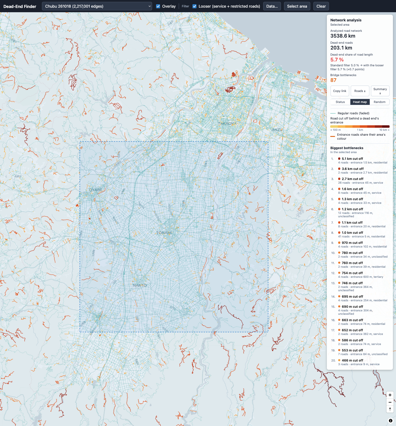
| Tonami (Japan) | 3,539 km | 203 km | 5.7% |
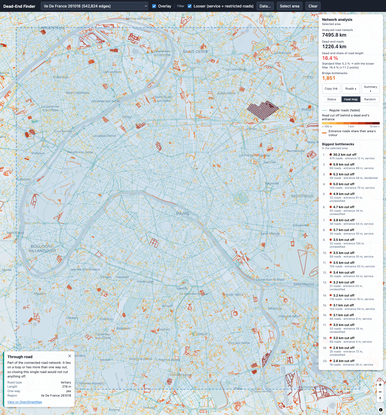
| Paris (France) | 7,496 km | 1,226 km | 16.4% |
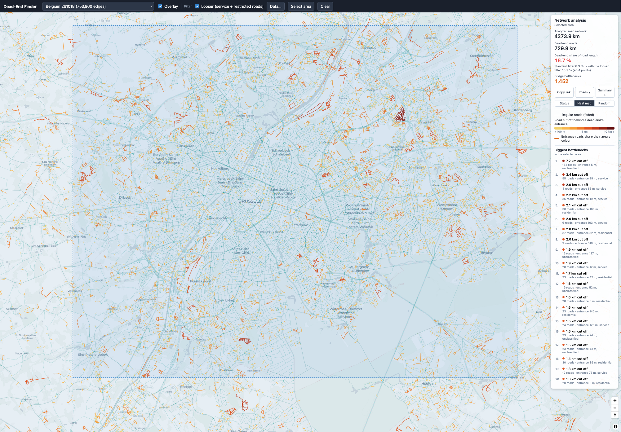
| Brussels (Belgium) | 4,374 km | 730 km | 16.7% |
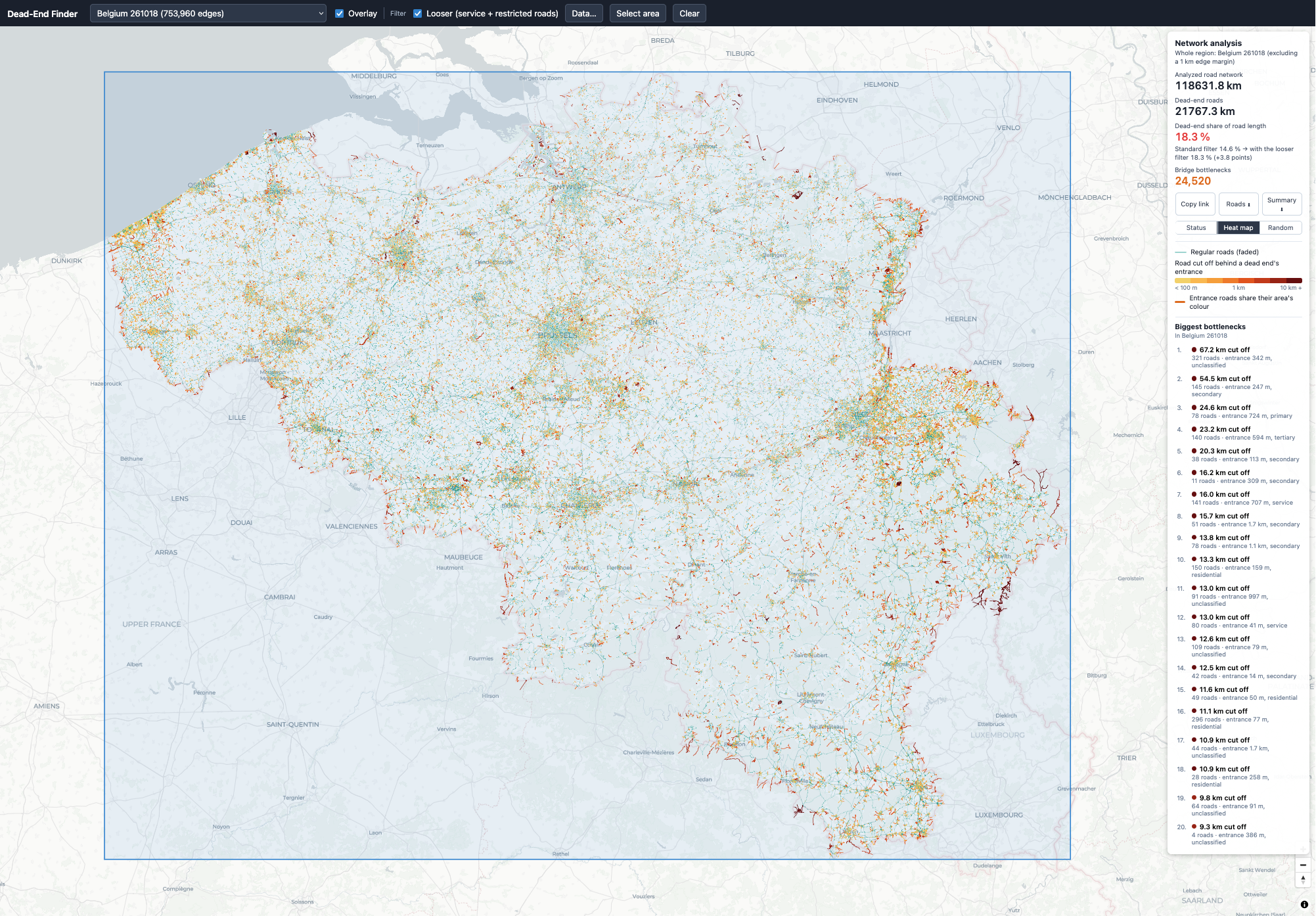
| Belgium (Entire Country) | 118,632 km | 21,767 km | 18.3% |
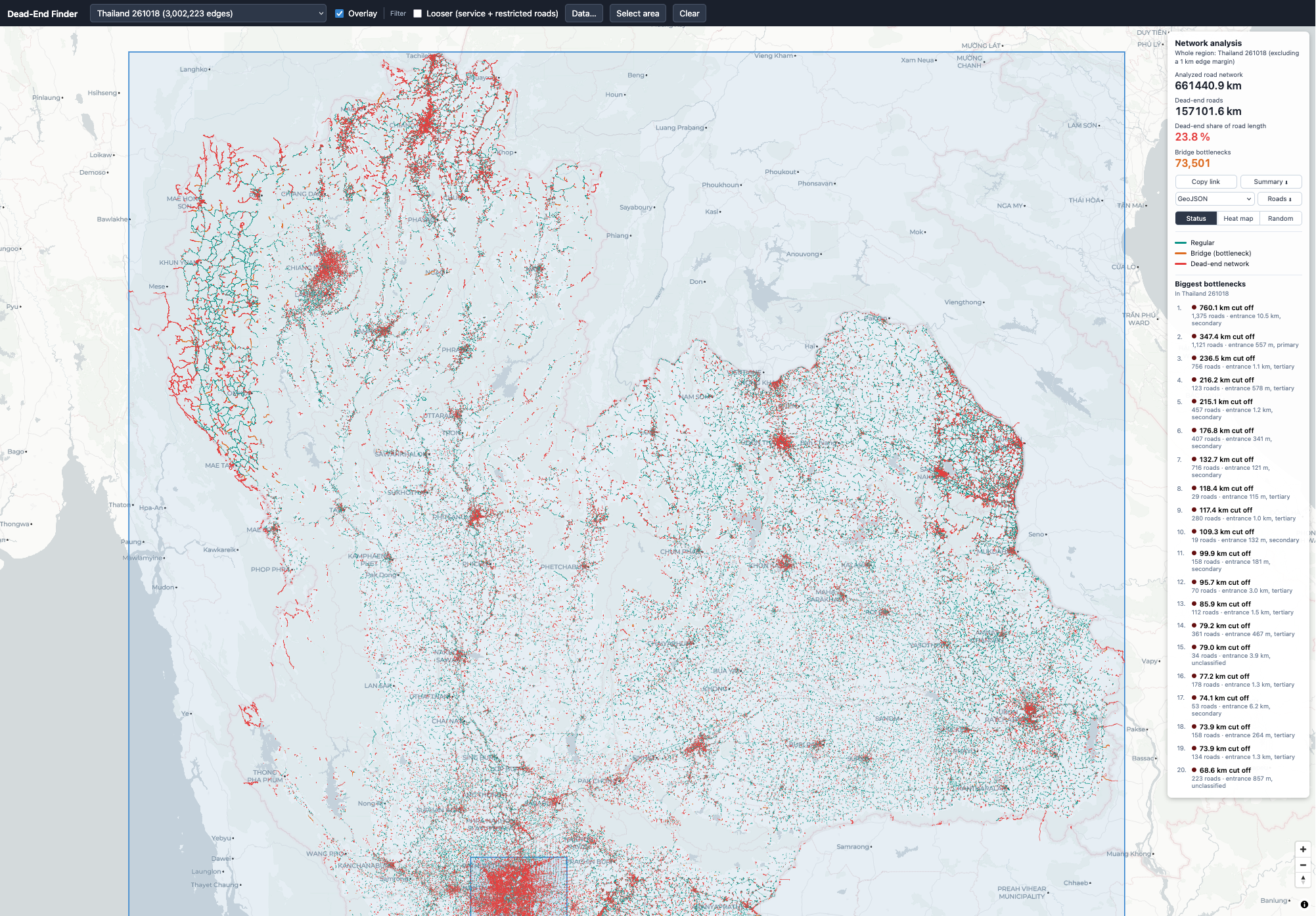
| Thailand (Entire Country) | 664,441 km | 157,102 km | 23.8% |
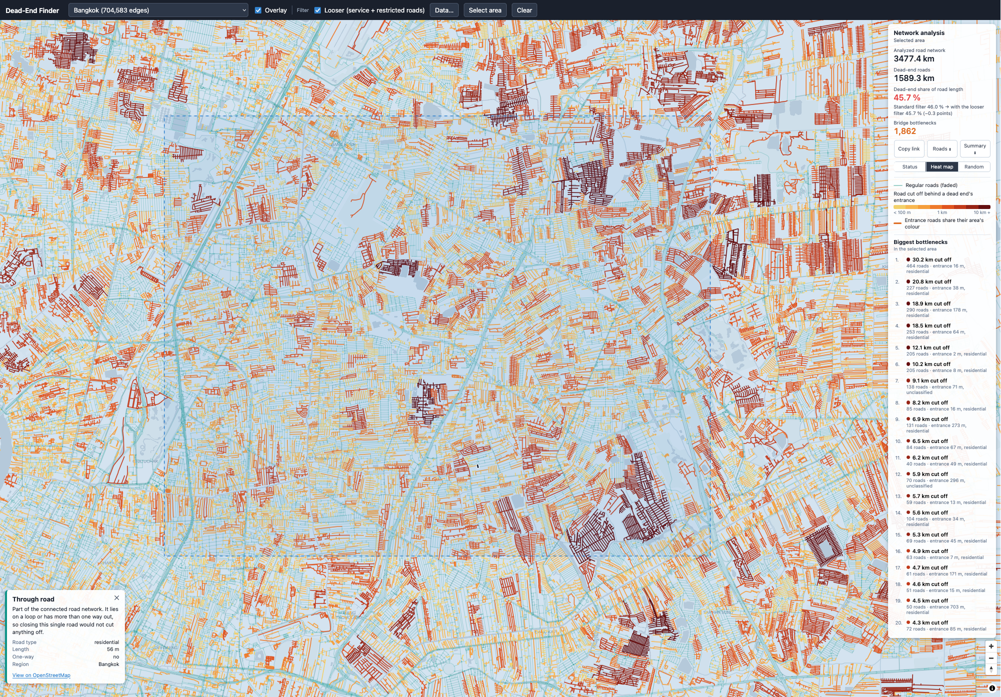
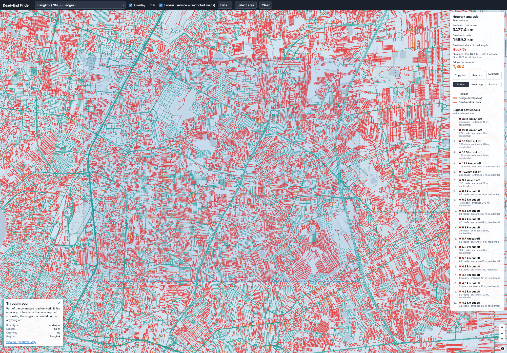
| Bangkok Neighborhood (Thailand) | 3,477 km | 1,589 km | 45.7% |
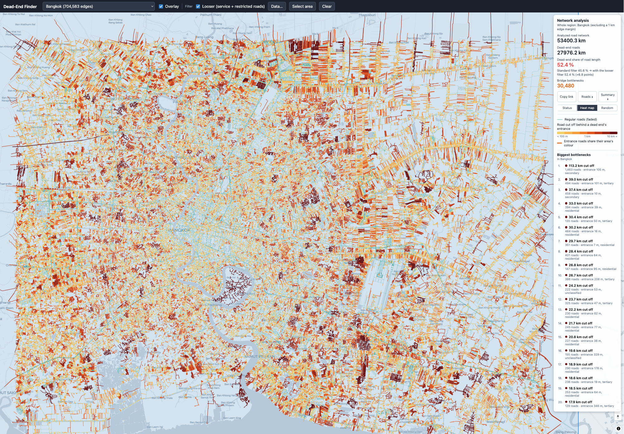
| Bangkok (Thailand) | 53,400 km | 27,976 km | 52.4% |
- The Grid vs. The Soi System: Tonami, Japan displays an exceptionally low dead-end ratio (5.7%) due to tight agricultural and urban grid planning. In stark contrast, Bangkok reaches a massive 52.4% dead-end ratio. This visually captures Bangkok’s famous soi (side-street) layout: long branching alleys that rarely connect laterally to adjacent neighborhoods, forcing nearly all traffic onto major avenues like Sukhumvit or Rama IV.
- European Medium Density: Cities like Paris and Brussels land in the 16–18% range. While old medieval centers have culs-de-sac and courtyard blocks, high perimeter density keeps overall through-way access strong.
These results seem to match my real-life experiences in those places I have visited.
Japanese city heat map
Paris heat map
Belgium heat map
Brussels heat map
Bangkok metropolitan area heat map
Zoomed analysis: Bangkok sub-district (heat map vs. vector classification)
Northern Thailand regional network map